Calculus, << KAL kyuh luhs, >> is the branch of mathematics that deals with changing quantities. Students usually learn it in college after they have mastered algebra, geometry, and trigonometry.
Calculus is the language in which engineers, physicists, and other scientists develop theories and solve practical problems. For example, the laws of aerodynamics are expressed in terms of calculus. An airplane designer can use these laws to calculate the changing forces that affect an airplane during flight. Calculus has also stimulated many new directions in mathematics since its development in the 1600’s.
Calculus was invented to answer questions that could not be solved using algebra or geometry. One branch of calculus, called differential calculus, began with questions about the speed of moving objects. For example, How fast does a stone fall two seconds after it has been dropped from a cliff? How fast is the earth moving around the sun on July 4? The other branch of calculus, integral calculus, was invented to answer a very different kind of question: What is the area of a shape with curved sides?
Although differential calculus and integral calculus began by solving different problems, their methods are closely related. The central problem of differential calculus is to find the rate at which a known, but varying, quantity changes. Integral calculus has just the reverse problem. It tries to find a quantity knowing the rate at which it is changing.
Differential calculus
Imagine an astronaut hovering in a landing craft near the surface of a planet with no atmosphere. Because of gravitational pull, a ball dropped from the craft will fall toward the planet. Through measurements, the astronaut finds that the ball falls 7 feet in 1 second, 28 feet in 2 seconds, and 700 feet in 10 seconds. Clearly, the ball is not falling at a constant speed. Using algebra, the astronaut determines the formula d = 7t2 for the distance (d) in feet that the ball falls from the landing craft in t seconds.
But assume that the astronaut wants to know the rate at which the ball’s distance from the landing craft is changing and so be able to determine the ball’s speed at any instant. Differential calculus can provide the astronaut with the formula s = 14t for the ball’s speed (s) in feet per second t seconds after it is dropped. Thus, the ball has a speed of 14 feet per second after 1 second, 28 feet per second after 2 seconds, and 140 feet per second after 10 seconds. From the formula s = 14t, differential calculus shows that the ball has a constant acceleration of 14 feet per second per second, written 14 ft/sec/sec or 14ft/sec2 . That is, in each second the speed of the ball increases 14 feet per second (14 ft/sec).
Functions.
Calculus deals with functions. A formula is often used to define a function. More precisely, a function (f) is a correspondence that associates with each number t some number f(t), read “f of t. ” For example, the formula d = 7t2 associates with each number t some number d. If we use f to label this function, then f(t) = 7t2. Thus, f(1) = 7 X 12 = 7, f(2) = 7 X 22 = 28, f(10) = 7 X 102 = 700.
Rate of change of a function
is the concern of differential calculus. If f(a) and f(b) are two values of the function f, then f(b) – f(a) equals the change in f brought about by the change from a to b in the number at which f is evaluated. The average rate of change of f between a and b is

The function f(t) = 7t2 describes the motion of the ball falling from the landing craft. The change in f from t = 2 to t = 10 equals f(10) – f(2) = 700 – 28 = 672. The average rate of change of f between 2 and 10 is

Thus, the ball falls 672 feet in 8 seconds, and the average speed of the ball during the 8-second period is 84 ft/sec. In a problem such as this where t is time and f(t) is distance, we use the term speed for the rate of change of f.
Limits.
Suppose a jet airplane makes a flight in which its average speed is 1,100 kilometers an hour. Also suppose that you wanted to know the speed of the airplane at any instant during its flight. You could not find this out by merely knowing the average speed of the jet. You would need other calculations.
Similarly, knowing the average speed of the ball dropped from the landing craft tells us little about its speed at any single instant. We need the idea of a limit to find this speed. Limits allow us to calculate the instantaneous rate of change of a function, such as the ball’s speed at a particular instant.
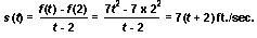
Consider the formula d = 7t2 for the distance the ball falls toward the planet in the situation already described. The average speed, s(t), of the ball between 2 seconds and t seconds after it is dropped is given by the following:
The following table of values gives the average speed of the ball over a time interval from 2 to t as the values of t get closer and closer to 2.
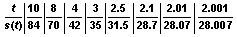
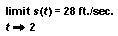
What is the average speed of the ball, s(t), close to when t is close to 2? From the table, we can clearly see that the answer is 28. In calculus, we would say that the limit of s(t) as t approaches 2 is 28 ft/sec. That is, the closer that t comes to 2, the closer the average speed comes to 28 ft/sec. The instantaneous speed of the ball 2 seconds after it is released is 28 ft/sec. In calculus, the fact that the instantaneous speed of the ball at t = 2 is 28 ft/sec is written:
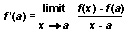
In general, the instantaneous rate of change of a function f at the number a is defined as follows:

Derivatives.
The instantaneous rate of change of a function is so important that mathematicians have given it the special name derivative. One of the most common symbols for the derivative of the function f at a is f′(a), which is read “f prime of a.” Other notations for the derivative are Dxf and df/dx. If we let y = f(x), then the notation dy/dx is used. The derivative is defined as follows:
All calculus books contain rules for finding derivatives of common functions. One of the most useful rules tells how to find the derivative of a power function, such as f(x) = cxn, where c is a constant. In this kind of function, f′(x) = cnxn – 1. This is the rule the astronaut should follow to find the speed of the falling ball. From f(t) = 7t2, it follows that f′(t) = 7 X 2t1 = 14t. Therefore, s = 14t is the formula for the speed of the ball at any time, t seconds, after it starts to fall.
Many functions can be shown as curved lines on a graph. At any point on a curve, we can draw a line tangent to the curve—that is, a straight line that touches the curve only at that point. The derivative provides the formula for the tangent line. The fact that the derivative is the slope of the tangent makes it a powerful tool for graphing functions.
Suppose we have a graph that shows the distance of the falling ball from the landing craft. The vertical axis of the graph indicates the distance (d) and the horizontal axis indicates the time (t). The curve of the graph shows us how the ball’s distance from the landing craft changes over time. The steepness, or slope, of the tangent line to the curve at any particular point is the ball’s speed at that instant.
Integral calculus
In physics, work is measured by the formula W = Fd, where W is the work done in foot-pounds, F is a constant force, and d is the distance through which the force acts. For example, if a constant force of 50 pounds is needed to push a box 20 feet across a room, then the work done is 20 X 50, or 1,000 foot-pounds. But if the force varies as the box is pushed, then the formula W = Fd does not apply. For example, you could not use the formula if the box was pushed with an ever-increasing force. But you could find the work done by using integral calculus. Integral calculus also solves many geometrical problems. For example, it is used to find the area of a region with a curved boundary. In fact, finding such areas is basic to integral calculus because it helps solve many problems, including the one of finding the work done by a variable force.
Finding areas.
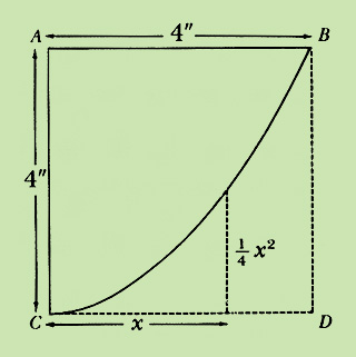
The curve BC shown below is part of a parabola, a shape commonly found in the reflectors of automobile headlights and in the mirrors used in telescopes. Suppose we want to find the area of the region BCD, which has sides BD and CD that are 4 inches long.
We can find the approximate area of BCD by drawing it on graph paper. In the graph below on the left, suppose the lines are 1 inch apart and each square therefore has an area of 1 square inch. In the graph below on the right, the lines are 1/2 inch apart and each square has an area of 1/4 square inch. In the bottom graph, the lines are 1/4 inch apart, and each square has an area of 1/16 square inch.
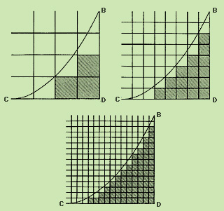
In the left-hand graph, BCD contains three squares with some area left over. Thus, BCD has an area of at least 3 square inches. In the right-hand graph, BCD contains 16 squares with some space left over. Since each square has an area of 1/4 square inch, BCD has an area of at least 4 square inches. In the bottom graph, each of the 74 small squares has an area of 1/16 square inch. Thus, BCD has an area of at least 45/8 square inches. If we kept plotting BCD on graph paper with smaller and smaller squares, we could get a closer approximation of its actual area. But we cannot get the exact area this way. Integral calculus does give us the exact area.
Here is a different way of approximating the area of BCD. Divide the line segment CD into eight parts, each 1/2 inch long. In the original parabola, any point on the parabola BC is 1/4x2 inches above the line CD at any point x inches from C. Using this fact, we find that the eight rectangles drawn in BCD have heights of 0, 1/16, 1/4, 9/16, 1, 25/16, 9/4, and 49/16 inches. The sum of their areas is given by the following: 
Thus, the area of BCD must be more than 43/8 square inches using this method.
If we divide the segment CD into n equal parts, where n is a positive whole number, each part has a length of 4/n inches. If we draw n rectangles in BCD just as we did above for n = 8, the sum, Sn, of the areas of the n rectangles is given by the following:
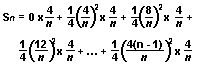
In this equation, the three dots indicate that some of the terms may have been left out. For example, if n = 100, 95 more terms should be included.
You can show by algebra that Sn = 16/3 – 8/n + 8/3n2.
As n gets larger and larger, the last two terms of this equation get closer and closer to 0. Thus, mathematicians say the limit of Sn as n approaches infinity (∞) is 16/3. They write this:

Since Sn is getting closer and closer to the area of BCD as n gets larger and larger, then the limit of Sn as n approaches infinity is the exact area of BCD. That is, the area of BCD is 16/3, or 51/3 square inches.
The definite integral.
A method similar to that used in the last example can be used to find the area of a more general region such as ABDC shown below.
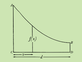
The area of ABDC may be approximated by drawing rectangles in it as we did for the parabola. The height of each rectangle is defined by the function f(x), which is the height of the curve x units from C. Therefore, if we draw four rectangles with equal bases, the sum of their areas is given by the following equation: 
In this equation, Δx (spoken “delta x”) equals d/4, the length of each base.
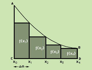
If we divide line segment CD into n equal parts by the points x0, x1, …, xn, and if we draw n rectangles in region ABDC, the sum, Sn, of the areas of the n rectangles is given by the following equation: 
Again, Δx = d/n, or the length of each base.
You can see that Sn is an approximation of the area of ABDC. As we divide line segment CD into more and more parts, making n larger and larger and Δx smaller and smaller, Sn becomes closer and closer to the actual area of ABDC. The actual area is the limit of Sn as n approaches infinity:

In words, a is the number that Sn is approaching as we divide segment CD into more and more parts, thereby making n larger and larger and Δx smaller and smaller.
The limit of Sn as n approaches infinity is called the definite integral of the function f from 0 to d. It is written with a stretched-out S as follows:

In this equation, dx indicates that a change in the value of x is the basis for change in the value of f(x).
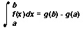
For a function f, defined between the numbers a and b where a is less than b, we can divide the segment between a and b into n equal parts and find the sum Sn as shown. The limit of Sn as n approaches infinity is called the definite integral of f from a to b and is written:

The fundamental theorem of calculus.
The area of a region with a curved boundary such as the area under the graph of a function f between the numbers a and b, can be found by a method that does not use the limits of sums of the areas of rectangles. First, suppose there is a function g that gives the area of the region between the numbers a and x. If we can find g, we can calculate the area between a and b. Mathematicians have discovered that the derivative of the function for the area, g′, always equals the function that defines the curve, f. This relationship is known as the fundamental theorem of calculus. It states that
where g is any function whose derivative is the function f. For example, f(x) = 1/4x2 is the height function of the parabola we have been studying. The function g, defined by g(x) = 1/12x3, has f as its derivative. This is because g′(x) = 1/123x2= 1/4x2 = f(x). By the fundamental theorem of calculus:
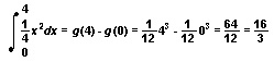
This is the area of region BCD under the parabola.
The fundamental theorem of calculus unites differential and integral calculus into one system that can solve a broad range of problems. The problem of finding an area becomes the problem of finding a function with a given derivative. The ability to find a function once the derivative is known enabled scientists to determine the speed of objects from the gravitational forces acting upon them. In the example of the falling ball, the speed increases by 14 feet each second, s = 14t. The fundamental theorem shows that the total distance the ball falls is given by the function whose derivative is s = 14t. That function is d = 7t2.
History
In solving problems of area, the Greek mathematician Archimedes used methods that foreshadowed those used today in integral calculus. In the 1600’s, differential calculus was developed in order to find tangents to curves and solve problems connected with the motions of planets and other objects. Then, the English scientist Sir Isaac Newton and the German philosopher Gottfried W. Leibniz independently discovered the fundamental theorem of calculus. For this discovery, Newton and Leibniz are called the founders of calculus.
See also Leibniz, Gottfried Wilhelm; Mathematics (History); Newton, Sir Isaac.